Computing exact distributions part 3
Integration and related ideas
I now review a general definition of integral. Although there are some techicalities the focus is on the main ideas.
Integration
Consider a function \(f\left( x \right)\) that is non-negative. The integral \(\int\limits_{\left( {a,b} \right)} {f\left( x \right)dx}\) is the area under the curve and above the horizontal axis in the interval \(\left( {a,b} \right)\). I will now look at this idea in more detail.
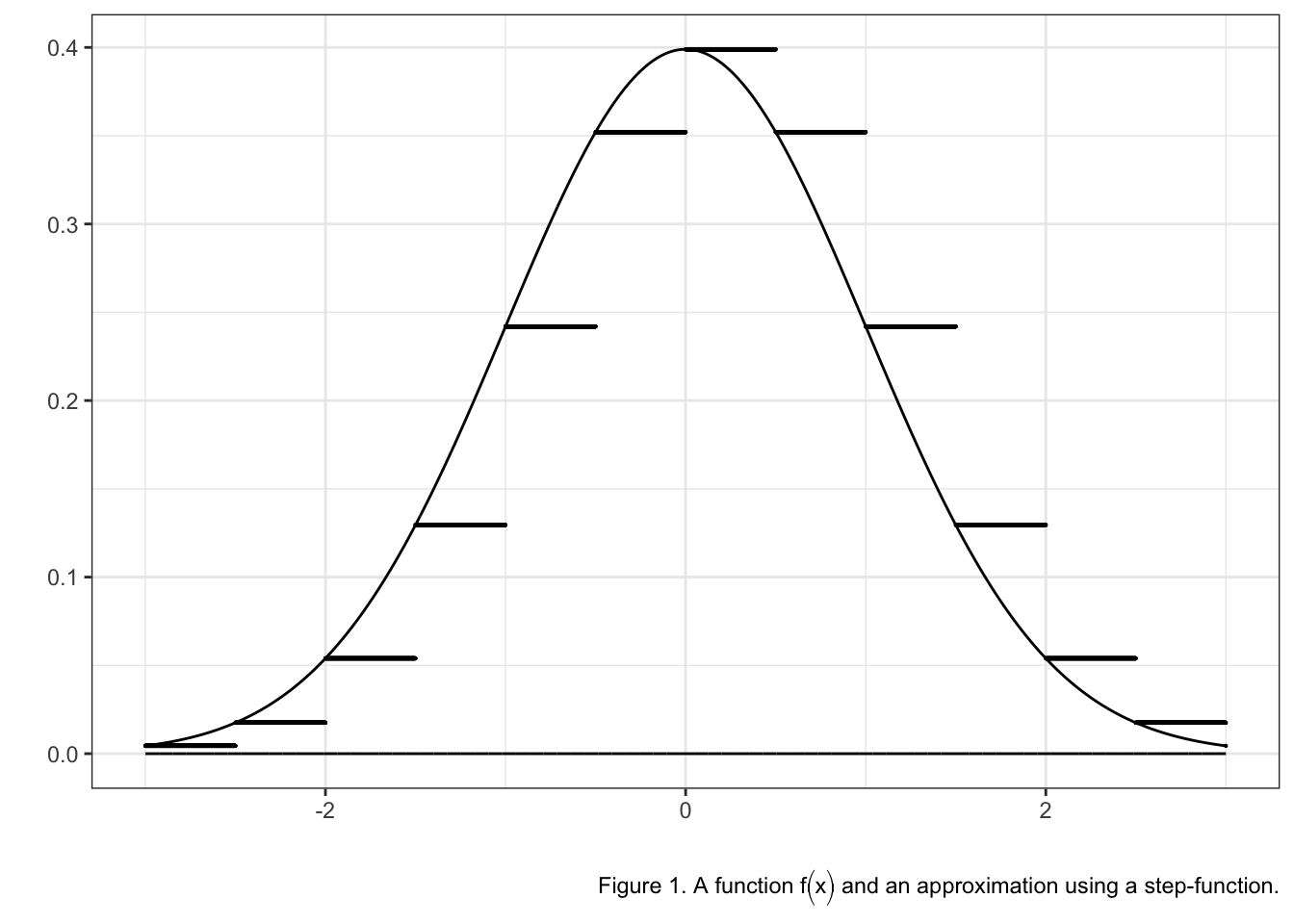
Any density function \(f\left( x \right)\) can be approximated by a step-function. To do this, I divide the interval \(\left[ {a,b} \right]\) into \(k + 1\) disjoint sub-intervals \(\left[ {{x_1},{x_2}} \right] = \left[ {a,{x_2}} \right]\), \(\left[ {{x_2},{x_3}} \right]\), \(\left[ {{x_3},{x_4}} \right]\), …., \(\left[ {{x_k},{x_{k + 1}}} \right] = \left[ {{x_k},b} \right]\), where \(a = {x_1} < {x_2} < {x_3} < ... < {x_k} < {x_{k + 1}} = b\), and define the step function \(f\left( x \right) = {x_j}\) when \(x \in \left( {{x_j},{x_{j + 1}}} \right)\). I can assume that all the intervals have the same length \(dx = {x_{j + 1}} - {x_j}\) for \(j = 1,2,...,k\). Figure 1 shows an example where the function \(f\left( x \right)\) is approximate by a step function in \(k = 10\) intervals.
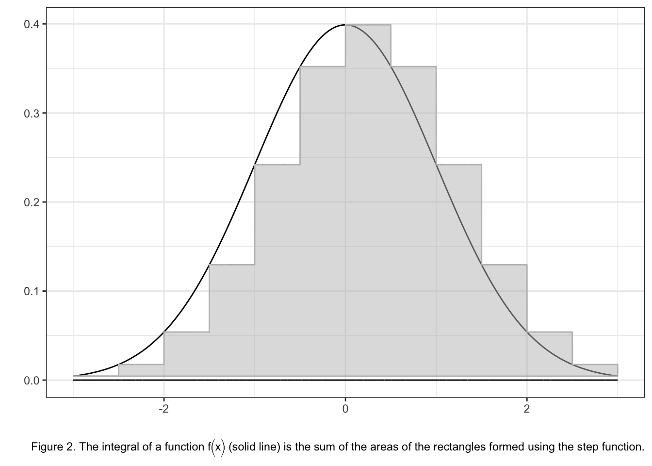
The integral of \(f\left( x \right)\) over the interval \(\left( {a,b} \right)\) is the area delimited by \(f\left( x \right)\), the horizontal axis, \(a\) and \(b\). It can be approximated by the sum of the areas of small rectangles as in Figure 2. So, formally I have, \[\begin{array}{c} \int\limits_{\left( {a,b} \right)} {f\left( x \right)dx} = \mathop {\lim }\limits_{k \to \infty } \sum\limits_{i = 1}^k {f\left( {{x_i}} \right)\left( {{x_{i + 1}} - {x_i}} \right)} \\ = \mathop {\lim }\limits_{k \to \infty } \sum\limits_{i = 1}^k {f\left( {{x_i}} \right)dx} . \end{array}\]
Notice that if \(f\left( x \right) = 1\) over \(\left( {a,b} \right)\)then \(\int\limits_{\left( {a,b} \right)} {1dx} = \int\limits_{\left( {a,b} \right)} {dx} = \mathop {\lim }\limits_{k \to \infty } \sum\limits_{i = 1}^k {dx} = b - a\) because the sum all small intervals is the length of the segment \(\left( {a,b} \right)\)
The concept of integral can be extended to functions that are not positive, but I do not need this because I will only deal with densities, and these are always positive. However, I need to extend the definition of integral to non-negative real functions \(f\left( x \right)\) where \(x = \left( {{x^1},{x^2},...,{x^n}} \right)\) is a vector in \(\mathbb{R}^n\).
Note that in our notation \({x^i}\) denotes the \(i\)-th component of \(x\) and not a power of \(x\). In this case the integral of \(f\left( x \right)\) over the set is the volume of the space between \(f\left( x \right)\) the n-dimensional space in which \(x\) lies and the contour of \(A\).
The set \(A\) can be approximated by small n-dimensional hyper-rectangles with sides \(d{x^1} = \left( {x_{{i_1} + 1}^1 - x_{{i_1}}^1} \right)\), \(d{x^2} = \left( {x_{{i_2} + 1}^2 - x_{{i_2}}^2} \right)\),…, \(d{x^n} = \left( {x_{{i_n} + 1}^n - x_{{i_n}}^n} \right)\), respectively.
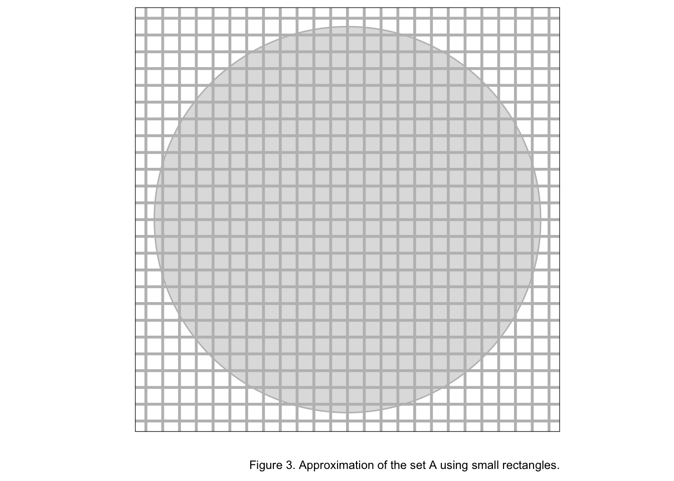
In Figure 3, the set \(A\) is represented by a circle. I can approximate \(A\) using small squares. Obviously, I need to consider only those squares that intersect \(A\).
The integral of \(f\left( x \right)\) over the set \(A\) and denoted by \(\int\limits_A {f\left( x \right)d{x^1}d{x^2}...d{x^n}}\) can be expressed as \[\begin{array}{c} \mathop {\lim }\limits_{k \to \infty } \sum\limits_{1 \le {i_1} \le k} {\sum\limits_{1 \le {i_2} \le k} {...\sum\limits_{1 \le {i_n} \le k} {f\left( {x_{{i_1}}^1,x_{{i_2}}^2,...,x_{{i_n}}^n} \right)\left( {x_{{i_1} + 1}^1 - x_{{i_1}}^1} \right)\left( {x_{{i_2} + 1}^2 - x_{{i_2}}^2} \right)....\left( {x_{{i_n} + 1}^n - x_{{i_n}}^n} \right)} } } \\ = \mathop {\lim }\limits_{k \to \infty } \sum\limits_{1 \le {i_1} \le k} {\sum\limits_{1 \le {i_2} \le k} {...\sum\limits_{1 \le {i_n} \le k} {f\left( {x_{{i_1}}^1,x_{{i_2}}^2,...,x_{{i_n}}^n} \right)d{x^1}d{x^2}...d{x^n}} } } \end{array}\] where the sum is over those squares that intersect \(A\) only.
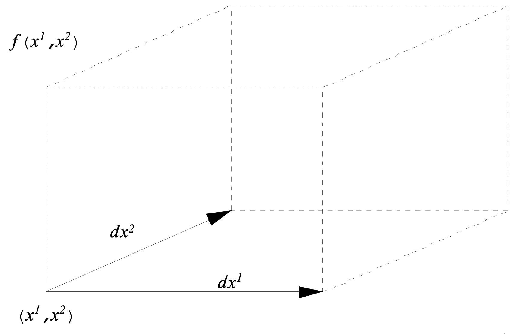
When \(n=2\), the term \(f\left( x_{i_1}^1,x_{i_2}^2 \right)dx^1 dx^2\) can be interpreted as the volume of the three-dimensional rectangle (cuboid or rectangular prism) with sides of length \(f\left( x_{i_1}^1,x_{i_2}^2 \right)\), \(d{x^1}\) and \(d{x^2}\). A geometric interpretation of all elements in the sum is given in Figure 4
Setting \(f\left( x \right) = 1\) over \(A\) gives \[\begin{array}{c} \int\limits_A {d{x^1}d{x^2}...d{x^n}} = \mathop {\lim }\limits_{k \to \infty } \sum\limits_{1 \le {i_1} \le k} {\sum\limits_{1 \le {i_2} \le k} {...\sum\limits_{1 \le {i_n} \le k} {d{x^1}d{x^2}...d{x^n}} } } \\ = {\text{Volume of }}A. \end{array}\]
The term \(d{x^1}d{x^2}...d{x^n}\) is often called the volume element because its integral determines the volume of the set \(A\). Notice that the expression \(d{x^i}\) is regarded as both the increment of \({x^i}\) and as a vector in \(\mathbb{R}^n\). I will use both these interpretations later on.
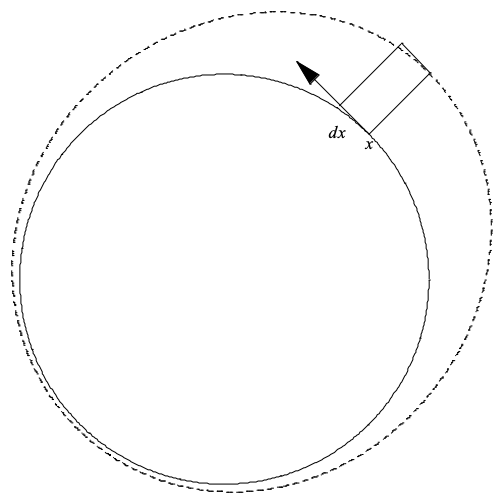
In some situation, I am interested in integrating non-negative functions defined on surfaces rather than planes. For example I could have a circle and a function defined on it as in Figure 5. To construct the integral in this case, I consider a set of \(k\) points on the circle. At each of these points I draw the tangent to the circle and construct small rectangles as illustrated in Figure 5. The integral is the limit of the sum of these rectangles as the number of points I consider on the circle goes to infinity. The generalization of these ideas to \(n\)-dimensional sphere is straightforward but a little bit messy.
Notice that I have already considered similar integrals when I looked at the Wishart distribution. In that case I integrated the density of the Wishart distribution over the set of positive definite matrices.
The change of variable formula and transformations
I now study how the integral changes when I transform the variable of integration according to the rule \(x = x\left( y \right)\). When I transform \(x\) to \(y\) I need this transformation to be one-to-one. That is, \(x\) transforms into one \(y\) and it is also possible to transform back \(y\) to \(x\) in a unique way.
I start by considering the case where \(n=1\).
In this case the integral is \(\int\limits_{\left( {a,b} \right)} {f\left( x \right)dx}\). I need to understand how this integral changes:
The interval \(\left( {a,b} \right)\) is transformed to the interval \(\left( {{a^*},{b^*}} \right)\) in such a way that \(x\left( {\left( {{a^*},{b^*}} \right)} \right) = \left( {a,b} \right)\).
The function \(f\left( x \right)\) changes to \(f\left( {x\left( y \right)} \right)\), and the volume element becomes \(dx\left( y \right) = x'\left( y \right)dy\).
Thus \[\int\limits_{\left( {a,b} \right)} {f\left( x \right)dx} = \int\limits_{\left( {{a^*},{b^*}} \right)} {f\left( {x\left( y \right)} \right)x'\left( y \right)dy}.\]
This is the transformation of variable formula for an integral.
Suppose for simplicity that \(f\left( x \right) = 1\) so that the integral I am interested in is \(\int\limits_{\left( {a,b} \right)} {dx}\), and suppose I transform \(x\) according to the rule \(x = y\) then \[\int\limits_{\left( {a,b} \right)} {dx} = \int\limits_{\left( {a,b} \right)} {dy} = b - a.\] If, instead, I transform \(x\) according to the rule \(x = - y\) I obtain \[\int\limits_{\left( {a,b} \right)} {dx} = \int\limits_{\left( { - a, - b} \right)} {\left( { - 1} \right)dy} = - \int\limits_{\left( { - a, - b} \right)} {dy} = - \left( { - b - \left( { - a} \right)} \right) = b - a.\]
Note that in this case the length of the interval \(\left( { - a, - b} \right)\) is \(\left( { - b - \left( { - a} \right)} \right) = - \left( {b - a} \right)\) because it is measured in the direction left to right, even though this integral is essentially the same as the one on \(\left( {a,b} \right)\).
We want to disregard these niggling problems with the sign so I want to transform \(\left( {a,b} \right)\) to \(\left( {{a^*},{b^*}} \right)\) with \({a^*} < {b^*}\) for any transformation. To be consistent with the definition of integral I need to transform the volume element to \[dx\left( y \right) = \left| {x'\left( y \right)} \right|dy\] where I take the absolute value of \(x'\left( y \right)\). In this notation, when I transform x according to the rule \(x = - y\) I obtain \[\int\limits_{\left( {a,b} \right)} {dx} = \int\limits_{\left( { - b, - a} \right)} {\left| { - 1} \right|dy} = \int\limits_{\left( { - b, - a} \right)} {dy} = \left( { - a - \left( { - b} \right)} \right) = b - a.\] This convention will be very useful when I look at multivariate integrals over a set \(A\) because I can disregard the direction along which the integral needs to be taken.
When I transform to according to \(x = x\left( y \right)\), then \(A\) changes to \({A^*}\) in such a way that \(A = x\left( {{A^*}} \right)\) and \(f\left( x \right)\) changes to \(f\left( {x\left( y \right)} \right)\). There are some small complications with the volume element. Notice that every component of \(x\) transforms as follows \({x_i} = {x_i}\left( {{y_1},{y_2},...{y_n}} \right)\). So the differential of \({x_i}\) is \[d{x_i} = \frac{{\partial {x_i}}}{{\partial {y_1}}}d{y_1} + \frac{{\partial {x_i}}}{{\partial {y_2}}}d{y_2} + ... + \frac{{\partial {x_i}}}{{\partial {y_n}}}d{y_n}\] for \(i=1,2,…,n\).
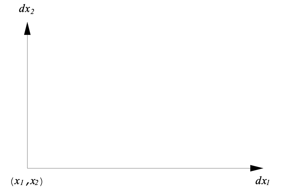
To analyse the problem I consider the case where \(n=2\). In this case \[\begin{array}{l} d{x_1} = \frac{{\partial {x_1}}}{{\partial {y_1}}}d{y_1} + \frac{{\partial {x_1}}}{{\partial {y_2}}}d{y_2}\\ d{x_2} = \frac{{\partial {x_2}}}{{\partial {y_1}}}d{y_1} + \frac{{\partial {x_2}}}{{\partial {y_2}}}d{y_2}. \end{array}\]
Notice that I have changed the notation slightly from \(dx^j\) do \(dx_j\), as this is more often used (above this notation would have been confusing).
Figure 6 gives a geometric interpretation of \(d{x_1}\) and \(d{x_2}\). I saw earlier on that \(d{x_1}d{x_2}\) is the area of the rectangle having \(d{x_1}\) and \(d{x_2}\) as sides. As I noted earlier on, the symbol \(d{x_i}\) can be interpreted as a \(2\)-dimensional vectors, \(d{x_i} = \left( {x_i^1,x_i^2} \right)\) say. The area of the rectangle having \(d{x_1}\) and \(d{x_2}\) as sides is just the determinant of \[\left| {\begin{array}{*{20}{c}} {d{x_1}}\\ {d{x_2}} \end{array}} \right| = \left| {\begin{array}{*{20}{c}} {x_1^1}&{x_1^2}\\ {x_2^1}&{x_2^2} \end{array}} \right|.\] The differentials above suggest that \[\left( {\begin{array}{*{20}{c}} {d{x_1}}\\ {d{x_2}} \end{array}} \right) = \left( {\begin{array}{*{20}{c}} {\frac{{\partial {x_1}}}{{\partial {y_1}}}}&{\frac{{\partial {x_1}}}{{\partial {y_2}}}}\\ {\frac{{\partial {x_2}}}{{\partial {y_1}}}}&{\frac{{\partial {x_2}}}{{\partial {y_2}}}} \end{array}} \right)\left( {\begin{array}{*{20}{c}} {d{y_1}}\\ {d{y_2}} \end{array}} \right).\]
Notice that \[\left| {\begin{array}{*{20}{c}} {d{x_1}}\\ {d{x_2}} \end{array}} \right| = \left| {\begin{array}{*{20}{c}} {\frac{{\partial {x_1}}}{{\partial {y_1}}}}&{\frac{{\partial {x_1}}}{{\partial {y_2}}}}\\ {\frac{{\partial {x_2}}}{{\partial {y_1}}}}&{\frac{{\partial {x_2}}}{{\partial {y_2}}}} \end{array}} \right|\left| {\begin{array}{*{20}{c}} {d{y_1}}\\ {d{y_2}} \end{array}} \right|,\] or in a different notation \[d{x_1}d{x_2} = \left| {\begin{array}{*{20}{c}} {\frac{{\partial {x_1}}}{{\partial {y_1}}}}&{\frac{{\partial {x_1}}}{{\partial {y_2}}}}\\ {\frac{{\partial {x_2}}}{{\partial {y_1}}}}&{\frac{{\partial {x_2}}}{{\partial {y_2}}}} \end{array}} \right|d{y_1}d{y_2}.\]
In general if I transform the variables according to the rules \(x = x\left( y \right)\) where to , then volume element \(d{x_1}d{x_2}....d{x_n}\) changes according to the rule \[d{x_1}d{x_2}....d{x_n} = J\left( {x \to y} \right)d{y_1}d{y_2}....d{y_n}\] where \(J\left( {x \to y} \right)\) denotes the Jacobian of the transformation of \(x\) to \(y\), and it is given by \[J\left( {x \to y} \right) = \left| {\left[ {\begin{array}{*{20}{c}} {\frac{{\partial {x_1}}}{{\partial {y_1}}}}&{\frac{{\partial {x_1}}}{{\partial {y_2}}}}& \cdots &{\frac{{\partial {x_1}}}{{\partial {y_n}}}}\\ {\frac{{\partial {x_2}}}{{\partial {y_1}}}}&{\frac{{\partial {x_2}}}{{\partial {y_2}}}}& \cdots &{\frac{{\partial {x_2}}}{{\partial {y_n}}}}\\ \vdots & \vdots & \ddots & \vdots \\ {\frac{{\partial {x_n}}}{{\partial {y_1}}}}&{\frac{{\partial {x_n}}}{{\partial {y_2}}}}& \cdots &{\frac{{\partial {x_n}}}{{\partial {y_n}}}} \end{array}} \right]} \right|,\] where in this case \(\left| . \right|\) denotes both the determinant and the absolute value.
To summarise, consider the probability of a set A \[\Pr \left\{ A \right\} = \int\limits_A {pdf\left( x \right)dx}\] and transform the variable of integration according to the rule \(x = x\left( y \right)\). I know that \[\Pr \left\{ A \right\} = \int\limits_{A'} {pdf\left( {x\left( y \right)} \right)J\left( {x \to y} \right)dy}\] where \(A = x\left( {A'} \right)\). So if \(pdf\left( x \right)\) is the density of x, and then transform \(x \to y\) then the density of y is \[pdf\left( y \right) = pdf\left( {x\left( y \right)} \right)J\left( {x \to y} \right).\] I now need to find ways for calculating the jacobian in more complex situations.